Using SHAP Values for Feature Importance
In this post I’d like to discuss Lundberg, Erion, and Lee’s 2019 paper “Consistent Individualized Feature Attribution for Tree Ensembles”, which can be found here. There are two main points of interest in this paper, and I’ll tackle both in order. First, how SHAP values are obtained and used in analyzing features in tree models and the advantages of doing so. Second, the tools that have been created to use SHAP values in practice.
What and Why?
Ensemble tree models may be powerful for making predictions, but they can be difficult to explain and interpret. In contrast with a basic decision tree model, ensemble models, like random forests or gradient boosted models, are “black box” models; they are not clearly explainable. Often our best option for attempting to understand our models is to determine the “feature importances” of the model. Notably this is the importance of features to the model, not the importance of features in general. Because feature importances will be both model specific and useful in comparing our models, we would like as robust and informative a way to do this as possible, and as a result multiple techniques have been created to do so.
The simplest way to get one of these measurements, in SciKit-Learn at least, is to just access .feature_importance_ on an ensemble tree model, which gives you the relevant values. As pretty much every bit of documentation for this attribute on sklearn will tell you, these values should be treated with caution. A more robust way of getting feature importances uses the permutation_importances function. This changes a single feature, scores the model again, and then compares. Rinse and repeat, and then you can get an idea of how important each feature is. SHAP values are another way to determine this information.
SHAP
To start with, a Shapley value is a game theory concept used to show the payoff each player can expect based on the value they provide in cooperative game. In other words, it shows how important each player is. Two of our authors published a paper in 2017 that shows that this concept can be extended to machine learning models with what they called SHAP (SHapley Additive exPlanation) values. Intuitively, this makes sense when viewing each prediction as an individual model. Each model is attempting to arrive at a prediction, and the members of the coalition (the set of players in the cooperative game) are the features the model is predicting on. Each feature can this way get a SHAP value, and we get the overall SHAP value of each feature in a data set by taking the mean of the individual SHAP values for each prediction.
Consistency
Building off that, the 2019 paper shows how SHAP can outperform most other current feature attribution methods used for tree models. In particular, the quality the authors most focus on is consistency. Unsurprisingly, in this context an inconsistency occurs when our importance metric is lower for a feature, while in reality it’s importance to the model has increased, most often due to reordering the model splits. Obviously this presents a major issue when attempting to explain models. Both SHAP and permutation importances are consistent, so now we can look at what else makes SHAP a desirable characteristic to use.
Individual vs. Global
As stated before, SHAP values for a feature are actually the mean of the SHAP values for that feature for each prediction, which of course means we can also look at single predictions. This is somewhat atypical for most ways of measuring feature importance for models: the authors noted that the only other metric they were aware that looked at individual predictions was Saabas. Saabas works in a similar way to the SciKit-Learn .feature_importance attribute mentioned earlier, and is similarly inconsistent and inaccurate. This individual assessment property has benefits for us when trying to plot the data, as we’ll see in a moment, but on it’s own it’s notable that SHAP can fulfill both roles in analysis.
Speed
Until this paper, SHAP values were difficult to compute efficiently. The authors have introduced an algorithm called Tree SHAP, which allows efficient SHAP values for ensemble models. This algorithm moves computation from O(2^M) time to O(D^2) time, with M as the number of features and D as the depth of the tree1. If you’re not familiar with big O notation, these represent the worst case running times for a basic algorithm and Tree SHAP respectively.
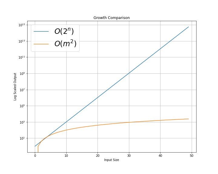
These are not the actual run time plots, but the worst cases for algorithms with O(2^n) and O(m^2). As can be seen, this is a significant run time improvement.
In Practice
Along with justifying the usage of SHAP values in feature evaluation, the authors also introduce their python module for this purpose. They’ve already included specific integrations with XGBoost and a number of other common ensemble modeling options, although as they point out, it’s possible to use the shap module with any model output. Of almost equal value to me, they also included quick plotting functions for their Explainer objects, to easily display the difference between features. Let’s take a look at this module by contrasting it the SciKit-Learn permutation_importance.
We’ll start by setting up a basic XGBoost model. I’m omitting the imports and some of the plotting code for later on, but all the code for this post can be found here.
data = load_breast_cancer()
X, y = data.data, data.target
X_train, X_test, y_train, y_test = train_test_split(X, y, random_state=42)

xgb_model = XGBClassifier().fit(X_train, y_train)
We can now set up our permutation importances:
result = permutation_importance(xgb_model, X_train, y_train, n_repeats=10, random_state=42)
perm_sorted_idx = result.importances_mean.argsort()
… and our SHAP explainer object. This object is the typical way to get information about our model. We also get the SHAP values base on our training data.
explainer = shap.Explainer(xgb_model)
shap_values = explainer(X_train)
We can compare the permutation importance:
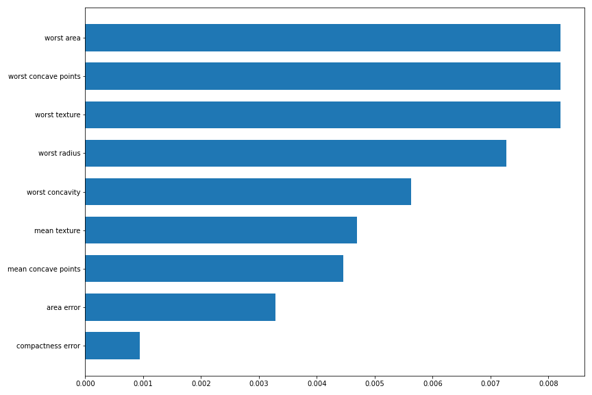
with the SHAP values:
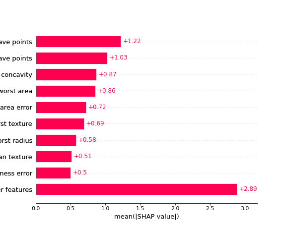
Now normally this is where we’d likely be satisfied if we were just using permutation importances, but SHAP has a few built in plots that take advantage of it’s individual prediction values, so we can take a look at a “bee swarm” plot:
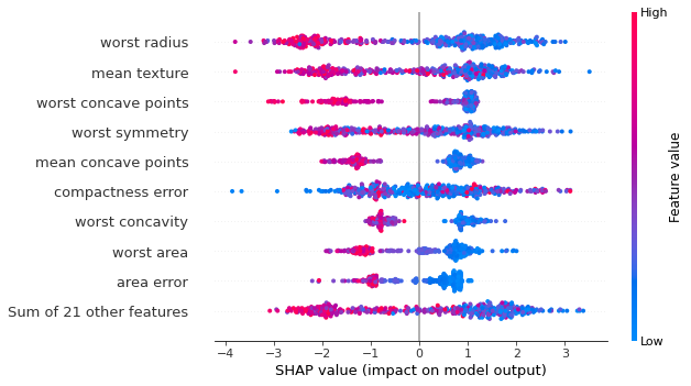
In this case, each dot is a SHAP value for a specific prediction, with it’s color indicating the actual value of a feature. This can help give us a clearer picture of how the features in our data change our model prediction. Conveniently, each of these plots needs only one line of code to call, for a seaborn-like usage. There are also many more types of plots depending on what you’re needs are.
How it all SHAPes up
It should be clear now that I consider Lundberg, Erion, and Lee’s argument to be very convincing; I highly encourage going to read the actual paper! They’ve shown that SHAP values are fast, consistent, and informative to use. In general having model evaluations with these qualities makes it easier to prove a model’s value, whether that’s to problem stakeholders, teachers, or anyone else who’s passing judgment on your model.
Thanks for reading! Please let me know if you have any suggestions or corrections, I’m always happy to retroactively appear more right than I was at the time!
Works Referenced
- Sklearn documentation examples: Feature importance, Permutation Importance
- A quick explanation of Shapley values
- The SHAP Documentation
- The SHAP GitHub Repository
- Lundberg and Lee’s 2017 Paper: A Unified Approach to Interpreting Model Predictions
- Shapley values on Wikipedia
- And of course, the topic paper for this post
-
The actual Big O notation used in the paper includes a few more terms, but I’m only using the ones that are different for clarity. ↩